Range Trees.

Introduction

I have been playing with implementing my old Liquid Cellular Automata using a discrete time simulation engine I implemented in Elixir. Basically it is a CA where the cells move around in a square and can only sense the state of other nearby cells. My biggest complaints about my original C++ implementation is that Identifying the neighbors of each cell is done in the least efficient way, by comparing the positions of all pairs of cells. This naive approach was “fast enough” at the time, but with a O(n²) running time it is deeply unsatisfying and kind of limits the scale of experiments that can be conducted. In my Elixir implementation I want to do better than O(n²). To do that I need to implement a data structure called a Range Tree that will enable searching for nearby cells in O(log² n + k) time where k is the number of cells returned from each query. With this data structure finding the neighbors of each cell in O(nlog² n + nk) time. In fact, I can use this data structure for points in an arbitrary number dimensions and each query will take O(logᵈ n + k) time where d is the number of dimensions. Fundamentally a range tree is just a balanced binary search tree with a fancier search function that returns a list of nodes instead of a single node.

For reasons of working in C++ before and, more importantly, premature optimization, I felt compelled to implement this data structure using balanced binary trees represented using the erlang array module. At some point it would actually be very interesting to compare the array representation with one that uses a more typical functional binary tree data structure like this

-type tree() :: {node, X :: float(), Left :: tree(), Right :: tree()}
              | {leaf, Value :: float()}.

Representing Binary Trees in Arrays

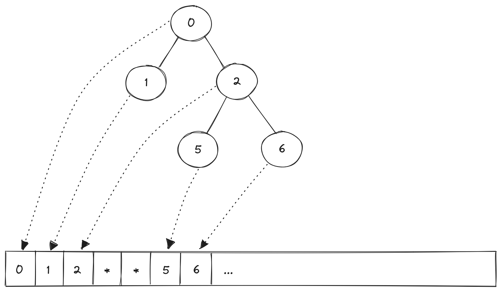
As a quick refresher, we can store a binary tree in an array and define the structure of the array with a clever indexing trick. Starting with the root of the tree at index i = 0, the left child is found at 2i + 1 and the right child is found at 2i + 2. This is shown in the image below. When there is no child present a special sentinel value is used to indicate that no node or leaf exists ("*" in the figure below).

One Dimensional Range Trees

I implemented a one-dimensional range tree first, since that made it easier to get the basic construction and search algorithms figured out. Once this is implemented it is fairly simple to extend it to multiple dimensions.

Construction

The tree will be stored in an erlang array. Each element of the array will hold either a node or a leaf which are just tagged tuples.

-type rangetree1() :: array:array({node | leaf, float(), pos_integer()}).

The second element of the tuple is the pivot value between the left and right children for nodes and the actual value of the point for leafs. The third value for nodes is the total number of leaves under that node. For leaf tuples, it is the index of the points position in the input used to construct the tree.

At a high level, constructing the tree is fairly simple. Given a list of points (floats, since this is one dimensional) we enumerate them to get their original position in the input list and then sort that list by the point value. A helper function build_tree/2 is used to construct nodes and leaves assign them to positions in the array. Finally the array is constructed from the list of nodes. The reason for returning a list of positions rather than constructing the array as we go is to limit the amount of extra memory allocation and garbage collection needed each time the array is modified. The approach I took here is vaguely inspired by the Repa array library for Haskell which provides a similar API for improving performance by collecting updates to individual positions of the array and applying them all at once in a batch.

-spec new([float()]) -> rangetree1().
new(Points) ->
    L = lists:keysort(2, enumerate(Points)),
    TList = build_tree(0, L),
    T = lists:keysort(1, lists:flatten(TList)),
    array:fix(array:from_orddict(T, undefined)).

The build_tree/2 function is only slightly more complex. As input it takes the array index where the top level node it produces should be stored and the sorted list of points that are below that node (remember the points have been enumerated, so they are actually tuples of an integer index and a float). build_tree returns a deep list of tuples containing the array index of the node and the node itself along with lists of tuples for all the points in the input list.

build_tree(RootIndex, [{N, X}]) -> [{RootIndex, {leaf, X, N}}];
build_tree(RootIndex, Points) ->
    {Left, Right} = split(Points),
    LeftTree = build_tree(RootIndex * 2 + 1, Left),
    RightTree = build_tree(RootIndex * 2 + 2, Right),
    {_, Median} = lists:last(Median),
    [{RootIndex, {node, X, length(Points)}}, LeftTree, RightTree].

If there is only one point in the list then a leaf is constructed storing the value of the point and its original index N. Otherwise, it the list of points is split into a lower half containing all points less than or equal to the median and an upper half containing all points greater than the median. Care is taken to ensure that if there are duplicate points at the median of the list they are all placed in the lower half. This is accomplished with the split/1 and split/3 functions.

split(List) ->
    split(length(List) div 2, List, []).

split(0, [{_, X} = H|List], [{_, X}|_] = L) ->
    split(0, List, [H|L]);
split(0, Right, Left) ->
    {lists:reverse(Left), Right};
split(N, [H|Rest], L) ->
    split(N - 1, Rest, [H|L]).

After splitting the list, the left sub-tree and right sub-tree are constructed recursively by passing 2i + 1 as the root index of the left and 2i + 2 as the root index of the right.

Once the deep list is returned to new/1 it is flattened and turned in to an array that enables fast-ish access to individual elements. In principle you could put the whole thing into an ETS table instead and get constant time access to each element if you wanted to.

In theory this construction method should take O(nlog n) time, but it might not be that good because of the split step which needs to traverse half the list, something that isn’t necessary if you are using arrays and pointers in C, for example. I haven’t actually figured out what that does to the running time yet; I tested it out with 1,000,000 points and it was fast enough¹ so I’m not worried about it.

Range Queries

Finding all the points in the range [x₀, x₁] requires two searches in the tree, one for each end of the range, then walking the tree between the result of those two searches and collecting all the leaves. The simplest way to do this (I think) is to find the node where the path from the root to x₀ and the path from the root to x₁ diverge. This node is called v-split. From v-split we continue down the left sub-tree, collecting all leaves to the right of each node on the path to x₀; we also continue down the right sub-tree to ox₁, collecting all the leaves to the left of each node on the path. Finally we decide whether to keep the leaves at the end of each path based on whether they fall into the range or not.

I implemented this using separate functions for each of those steps: find_vsplit, collect_left, and collect_right.

find_vsplit(Min, Max, Tree, I) ->
    case array:get(I, Tree) of
        {node, X, _} when X < Max, Min =< X ->
            %% The paths diverge here, this is VSplit
            I;
        {node, X, _} when Max =< X ->
            %% the range is contained on the left
            find_vsplit(Min, Max, Tree, 2 * I + 1);
        {node, X, _} when X < Min ->
            %% the range is contained on the right
            find_vsplit(Min, Max, Tree, 2 * I + 2);
        {leaf, _, _} ->
            %% If we reached a leaf then that is VSplit
            I
    end.

collect_left(Max, Tree, I) ->
    case array:get(I, Tree) of
        {leaf, X, N} when X =< Max ->
            [N];
        {leaf, _, _} ->
            [];
        {node, X, _} when X < Max ->
            collect_left(Max, Tree, 2 * I + 2) ++ leaves(2 * I + 1, Tree);
        {node, X, _} when X >= Max ->
            collect_left(Max, Tree, 2 * I + 1)
    end.

collect_right(Min, Tree, I) ->
    case array:get(I, Tree) of
        {leaf, X, N} when Min =< X ->
            [N];
        {leaf, _, _} ->
            [];
        {node, X, _} when Min =< X ->
            collect_right(Min, Tree, 2 * I + 1) ++ leaves(2 * I + 2, Tree);
        {node, X, _} when Min > X ->
            collect_right(Min, Tree, 2 * I + 2)
    end.

The function leaves/2 is used to collect all leaves below a specific index.

leaves(I, Tree) ->
    case array:get(I, Tree) of
        {leaf, _, N} ->
            [N];
        {node, _, _} ->
            leaves(2 * I + 1, Tree) ++ leaves(2 * I + 2, Tree)
    end.

Finally query/3 orchestrates these three functions to perform a range query, first finding the index of v-split and then collecting the leaves in the range on its left and right sub-trees.

-spec query(Min :: float(), Max :: float(), Tree :: rangetree1()) -> [pos_integer()].
query(Min, Max, Tree) when Min =< Max ->
    VSplit = find_vsplit(Min, Max, Tree, 0),
    case array:get(VSplit, Tree) of
        {leaf, X, N} when Min =< X, X =< Max ->
            [N];
        {leaf, _, _} ->
            [];
        {node, _, _} ->
            Lower = collect_right(Min, Tree, 2 * VSplit + 1),
            Upper = collect_left(Max, Tree, 2 * VSplit + 2),
            Lower ++ Upper
    end.

Testing with PropEr

This seemed like a great opportunity to try out proper. There are a lot of edge cases that I could test manually, but what I really want is to test that when a range query is executed, every value returned lies in the range and every value not returned lied outside the range. I did this using two properties.

-module(prop_rangetree1).
-include_lib("proper/include/proper.hrl").

%%%%%%%%%%%%%%%%%%
%%% Properties %%%
%%%%%%%%%%%%%%%%%%
prop_all_covered_in_range() ->
    ?FORALL({Points, {Min, Max}}, {points(), range()},
        begin
            T = rangetree1:new(Points),
            Covered = rangetree1:query(Min, Max, T),
            {CoveredValues, _NotCoveredValues} = partition_values(Points, Covered),
            lists:all(fun(X) -> (Min =< X) and (X =< Max) end, CoveredValues)
        end).

prop_all_not_covered_out_of_range() ->
    ?FORALL({Points, {Min, Max}}, {non_empty(list(float())), range()},
        begin
            T = rangetree1:new(Points),
            Covered = rangetree1:query(Min, Max, T),
            {_CoveredValues, NotCoveredValues} = partition_values(Points, Covered),
            lists:all(fun(X) -> (X > Max) or (X < Min) end, NotCoveredValues)
        end).

%%%%%%%%%%%%%%%
%%% Helpers %%%
%%%%%%%%%%%%%%%
partition_values(Points, Covered) ->
    {[lists:nth(N, Points) || N <- Covered],
     [lists:nth(N, Points) || N <- (lists:seq(1, length(Points)) -- Covered)]}.

%%%%%%%%%%%%%%%%%%
%%% Generators %%%
%%%%%%%%%%%%%%%%%%
points() ->
    non_empty(list(float())).

range() ->
    ?SUCHTHAT({Min, Max}, {float(), float()}, Min =< Max).

Multi-dimensional Range Tree

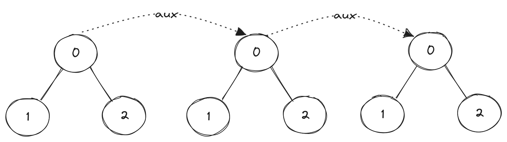
A multi-dimensional range tree is fundamentally a collection of one-dimensional range trees build using coordinates for each dimension. We could do this by building one range tree for each dimension, querying each of them individually, and returning the intersection of the results; however, this is not the most time-efficient approach. Instead of one extra range tree per dimension we will construct n - 1 additional range trees, one for each node in the one-dimensional range tree. This lets us narrow down the search in the d-th dimension to only include those points we know are within range for dimension d-1, but at the cost of additional memory usage since there is substantial duplication of the input data within the trees.

To build a multi-dimensional range tree we need to modify the structure of the nodes. Instead of storing the size of the tree rooted at each node, we will store an auxiliary tree containing the same nodes, but sorted on the “next” dimension. If there is no next dimension we will just store nil. The figure below shows what a 3 dimensional tree with two points looks like.

To construct this we follow the same basic algorithm used for the one dimensional tree: sort the points by their d-th coordinate, find the median, add a node and proceed recursively with the left and right children. However, we must add an extra step: for each node we create an entirely new range tree using just the coordinates for dimensions d + 1 to D (where D is the number of dimensions). When we get to a one-dimensional coordinate we stop.

-type rangetree() :: array:array({node, float(), nil | rangetree()} |
                                 {leaf, float(), pos_integer()}).

-spec new([[float()]]) -> rangetree().
new(Points) ->
    new_tree(enumerate(Points)).

new_tree(Points) ->
    L = lists:sort(
          fun ({_, [X|_]}, {_, [Y|_]}) ->
                  X =< Y
          end,
          Points),
    TList = build_tree(0, L),
    T = lists:keysort(1, lists:flatten(TList)),
    array:fix(array:from_orddict(T, undefined)).

split(List) ->
    split(length(List) div 2, List, []).

split(0, [{_, [X|_]} = H|List], [{_, [X|_]}] = L) ->
    split(0, List, [H|L]);
split(0, Right, Left) ->
    {lists:reverse(Left), Right};
split(N, [H|Rest], L) ->
    split(N - 1, Rest, [H|L]).

build_tree(RootIndex, []) -> [{RootIndex, undefined}];
build_tree(RootIndex, [{N, [X|_]}]) -> [{RootIndex, {leaf, X, N}}];
build_tree(RootIndex, Points) ->
    {Left, Right} = split(Points),
    LeftTree = build_tree(RootIndex * 2 + 1, Left),
    RightTree = build_tree(RootIndex * 2 + 2, Right),
    {_, [X|_]} = lists:last(Left),
    [{RootIndex, {node, X, build_aux(Points)}}, LeftTree, RightTree].

build_aux([{_, [_]}|_]) -> nil;
build_aux(Points)       -> new_tree([{I, T} || {I, [_|T]} <- Points]).

In the new version the coordinates of each point are represented by a list of floats. The function build_aux/1 is used to recursively build a new range tree on the tail of each coordinate list, up until there is only one dimension. Note that we added a new function new_tree/1 that expects the enumerated points as input since we don’t want to create a new (and incorrect) enumeration for each auxiliary tree.

Multi-dimensional Range Queries

Queries on the multi-dimensional tree are almost identical to the one-dimensional tree. The only exception is the query/3 function. This function now has an extra recursive step where the auxiliary tree at v-split is queried for the next dimension. The return value is the intersection of this recursive call and the set of leaves returned from the left and right children.

-spec query(Min :: [float()], Max :: [float()], Tree :: rangetree()) ->
          [pos_integer()].
query([], [], _) -> [];
query([Min|MinRest], [Max|MaxRest], Tree) ->
    VSplit = find_vsplit(Min, Max, Tree, 0),
    case array:get(VSplit, Tree) of
        {leaf, X, N} when Min =< X, X =< Max ->
            [N];
        {leaf, _, _} ->
            [];
        {node, _, Aux} ->
            Lower = collect_right(Min, Tree, 2 * VSplit + 1),
            Upper = collect_left(Max, Tree, 2 * VSplit + 2),
            AuxI = sets:from_list(query(MinRest, MaxRest, Aux)),
            D = sets:from_list(Lower ++ Upper),
            sets:to_list(sets:intersection([AuxI, D]))
    end.

Testing with PropEr

The two properties we test for the multi-dimensional tree are the same as the properties for the one-dimensional tree. The only difference is that we do a little extra work to compare each dimension’s coordinate. The major difference for the multi-dimensional tree is that we need more complex generator functions to yield points that all have the same dimensionality.

-module(prop_rangetree).
-include_lib("proper/include/proper.hrl").

%%%%%%%%%%%%%%%%%%
%%% Properties %%%
%%%%%%%%%%%%%%%%%%
prop_all_covered_in_range() ->
    ?FORALL({Points, {Min, Max}}, tree_and_query(),
        begin
            T = rangetree:new(Points),
            Covered = rangetree:query(Min, Max, T),
            {CoveredValues, _NotCoveredValues} = partition_values(Points, Covered),
            lists:all(
              fun(P) -> lists:any(
                          fun({X, XMin, XMax}) -> (XMin =< X) and (X =< XMax) end,
                          lists:zip3(P, Min, Max))
              end, CoveredValues)
        end).

prop_all_not_covered_out_of_range() ->
    ?FORALL({Points, {Min, Max}}, tree_and_query(),
        begin
            T = rangetree:new(Points),
            Covered = rangetree:query(Min, Max, T),
            {_CoveredValues, NotCoveredValues} = partition_values(Points, Covered),
            lists:all(
              fun(P) -> lists:any(
                          fun({X, XMin, XMax}) -> (X < XMin) or (X > XMax) end,
                          lists:zip3(P, Min, Max))
              end, NotCoveredValues)
        end).

%%%%%%%%%%%%%%%
%%% Helpers %%%
%%%%%%%%%%%%%%%
partition_values(Points, Covered) ->
    {[lists:nth(N, Points) || N <- Covered],
     [lists:nth(N, Points) || N <- (lists:seq(1, length(Points)) -- Covered)]}.

%%%%%%%%%%%%%%%%%%
%%% Generators %%%
%%%%%%%%%%%%%%%%%%
dimensions() ->
    ?LET(D, integer(), (abs(D) rem 10) + 1).

tree_and_query() ->
    ?LET(Dims, dimensions(), {points(Dims), range(Dims)}).

points(Dims) ->
    ?LET(D, Dims, non_empty(list(point(D)))).

point(Size) ->
    [float() || _ <- lists:seq(1, Size)].

range(Dims) ->
    ?LET({Xs, Ys}, {point(Dims), point(Dims)},
         {lists:zipwith(fun min/2, Xs, Ys), lists:zipwith(fun max/2, Xs, Ys)}).

There is a bug in the rangetree:query/3 function that provides a good reminder that we should be careful with properties. Despite the bug, which causes the function to always return [], the prop_all_covered_in_range property passes. This property is really only useful in conjunction with the prop_all_not_covered_out_of_range property which makes me think it would be a better idea to combine these into one property.

To fix the bug we just need to change the base case for the query/3 function. It was originally implemented to recursively call itself until the dimensions of its input range are exhausted. Unfortunately that means the end of the recursion is always []; when we take the intersection of an empty set with anything we always get an empty set. (This is why the first property passes—everything in the empty set is within the range.) Instead of basing the recursion on the input range, we need to use the absence of an aux tree as a signal that the recursion should stop because there are no more dimensions. The corrected function is listed below.

-spec query(Min :: [float()], Max :: [float()], Tree :: rangetree()) ->
          [pos_integer()].
query([Min|MinRest], [Max|MaxRest], Tree) ->
    VSplit = find_vsplit(Min, Max, Tree, 0),
    case array:get(VSplit, Tree) of
        {leaf, X, N} when Min =< X, X =< Max ->
            [N];
        {leaf, _, _} ->
            [];
        {node, _, nil} ->
            Lower = collect_right(Min, Tree, 2 * VSplit + 1),
            Upper = collect_left(Max, Tree, 2 * VSplit + 2),
            Lower ++ Upper;
        {node, _, Aux} ->
            Lower = collect_right(Min, Tree, 2 * VSplit + 1),
            Upper = collect_left(Max, Tree, 2 * VSplit + 2),
            AuxI = sets:from_list(query(MinRest, MaxRest, Aux)),
            D = sets:from_list(Lower ++ Upper),
            sets:to_list(sets:intersection([AuxI, D]))
    end.

Conclusion

I will follow this post up with another one measuring the performance of this range tree relative to the naive all-pairs comparison approach to the problem described in the introduction. It should be faster, but either way it was fun to implement. I may also compare this implementation to one that doesn’t use arrays; I really am not sure what the difference in performance will be, but it is possible that the array implementation actually performs worse. No way to know until I measure it.

All the code for this post can be found on my github.